Path Planning Algorithms

Unique Algorithms

Path Planning Algorithms

Comprehensive path planning implementation featuring Bi-Directional Rapidly-exploring Random Trees (Bi-RRT) and Artificial Potential Field (APF) methods for robot navigation in complex environments.

Path Planning Visualizations

Algorithm Overview

Path planning is fundamental to robotics and autonomous systems, determining optimal collision-free paths from start to goal positions while respecting environmental constraints and kinematic limitations.

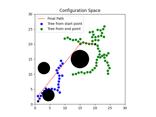
Bi-Directional RRT

An efficient sampling-based algorithm that grows two trees simultaneously from start and goal positions, significantly improving convergence speed over traditional single-tree RRT.

Algorithm Principles

Bi-RRT operates on the principle of dual exploration:

• Simultaneous Tree Growth: Two trees expand from start and goal positions
• Random Sampling: Generates random configurations in configuration space
• Tree Connection: Attempts to connect trees when they approach each other
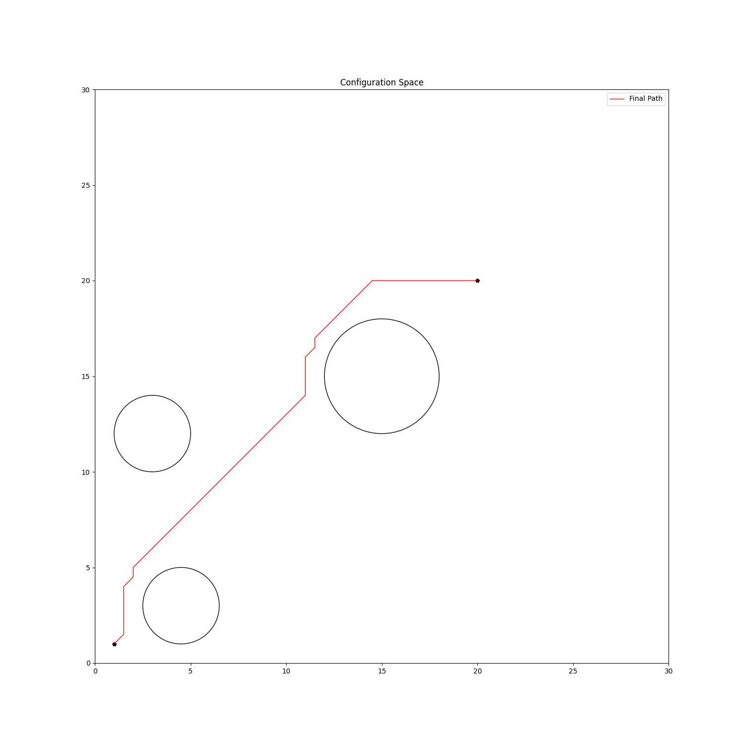
• Path Extraction: Once connected, extracts complete path

Mathematical Foundation

The algorithm explores configuration space C using random sampling:

$$q_{rand} \sim U(C_{free})$$

Tree expansion follows:

$$q_{new} = q_{near} + \alpha \cdot \frac{q_{rand} - q_{near}}{|q_{rand} - q_{near}|}$$

Where $\alpha$ is the step size parameter.

Implementation Details

# Bi-RRT execution with custom iterations
python bi_rrt.py --iter 200

# Default configuration (100 iterations)
python bi_rrt.py

Artificial Potential Fields

A physics-inspired approach that models the environment as potential fields, where obstacles generate repulsive forces and the goal generates attractive forces.

Potential Field Theory

The total potential at any point q is the superposition:

$$U(q) = U_{att}(q) + \sum_{i=1}^{n} U_{rep_i}(q)$$

Where:

• $U_{att}(q)$ is the attractive potential from the goal
• $U_{rep_i}(q)$ is the repulsive potential from obstacle i

Attractive Potential Functions

Two formulations are supported:

Parabolic Function:

$$U_{att}(q) = \frac{1}{2} \kappa |q - q_{goal}|^2$$

Conical Function:

$$U_{att}(q) = \kappa |q - q_{goal}|$$

Repulsive Potential

For obstacle i with distance $d_i = |q - q_{obs_i}|$:

$$U_{rep_i}(q) = \begin{cases} \frac{1}{2} \eta \left(\frac{1}{d_i} - \frac{1}{Q}\right)^2 & \text{if } d_i \leq Q \\ 0 & \text{if } d_i > Q \end{cases}$$

Where $Q$ is the influence distance and $\eta$ is the repulsive gain.

Implementation

# Custom configuration
python pf.py --grid 0.5 --function conical --attractive 1 --repulsive 5000

# Default settings
python pf.py

Streamlit Visualization

Interactive web-based visualization using Streamlit for real-time algorithm demonstration and parameter tuning.

Features

• Real-time Visualization: Watch algorithms explore the space
• Parameter Adjustment: Modify algorithm parameters during execution
• Multiple Algorithms: Switch between Bi-RRT and APF methods
• Environment Customization: Define custom obstacle configurations
• Path Analysis: Examine generated paths and algorithm performance

Launch Interface

streamlit run app.py

Algorithm Comparison

Different path planning approaches offer distinct advantages for various scenarios.

Bi-RRT Characteristics

Advantages:

• Probabilistic Completeness: Guaranteed to find a path if one exists
• High-Dimensional Support: Works well in complex configuration spaces
• Fast Convergence: Bidirectional search improves efficiency
• Optimality: Can approach optimal solutions with sufficient iterations

Limitations:

• Non-Deterministic: Path quality varies between runs
• Parameter Sensitivity: Performance depends on step size and iterations
• Memory Usage: Tree structures can grow large

APF Characteristics

Advantages:

• Deterministic: Reproducible paths for given configurations
• Real-time Capability: Suitable for dynamic environments
• Smooth Paths: Naturally generates smooth trajectories
• Local Optimality: Converges to local minima

Limitations:

• Local Minima: Can get trapped in non-optimal solutions
• Narrow Passage Difficulty: Struggles with tight corridors
• Parameter Tuning: Requires careful gain selection
• Completeness Issues: Not guaranteed to find paths

Applications

• Mobile Robotics: Autonomous navigation in unknown environments
• Manipulator Planning: Robot arm trajectory planning
• Autonomous Vehicles: Self-driving car path planning
• Game AI: Non-player character navigation
• Aerospace: Aircraft trajectory optimization

Technical Requirements

pip install -r requirements.txt

Dependencies include NumPy for numerical computations, Matplotlib for visualization, and Streamlit for the interactive interface.

Implementation Notes

The modular design allows easy extension with additional algorithms and supports both 2D and 3D planning spaces with minimal modification.